Chapter 3 Single-cell RNA-seq Data Processing and Quality Control

Once the raw data is obtained, the first thing to do is to check the quality of the reads and process it accordingly. In this chapter, we will go through quality control and processing methods for single-cell data.

3.1 Cell Ranger Pipeline

FIGURE 3.1: Cell Ranger Pipeline (2019)

In 10X Genomics workflow, which is the main workflow that is commonly used nowdays, Cell Ranger pipeline is used to process Chromium single-cell data to generating feature-barcode matrices, reading alignment, filtering, clustering and perform other secondary analysis methodologies.(2019)

Cell Ranger identifies each sample, cell and molecule. Identification done by using sequencing barcodes (eg. Illumina i7 and i5 indices) for samples, cell-specific barcodes for cells and, UMIs for molecules. The typical Cell Ranger results looks like this:

FIGURE 3.2: Cell Ranger Pipeline Results (2019)

In the previous chapter, we mentioned that some of the droplets may contain no cells. In the qc summary report of the Cell Ranger pipeline, Cell Ranger predicts the number of cells within the inputed data and print the estimation in “Estimated Number of Cells” section. The “Barcode Rank Plot” indicates the droplets that contains bead but no cell with the grey color. To determine a cut-off and remove noisy data, bioinformaticians benefit from this plot. The “Mapping” section of the report indicates percantage of reads that is aligned successfully to the genome.

• HINT : If the mapping rate is low and, you are working with the pure data (eg. human data) that may indicate contamination.

• NOTE : Cell Ranger prints error, if there is a quality issue.

3.1.1 FASTQ File Format

High-throughput sequencing reads usually outputs FASTQ files. Cell Ranger pipeline produces FASTQ files as well. Let’s take a look at the FASTQ file format below.

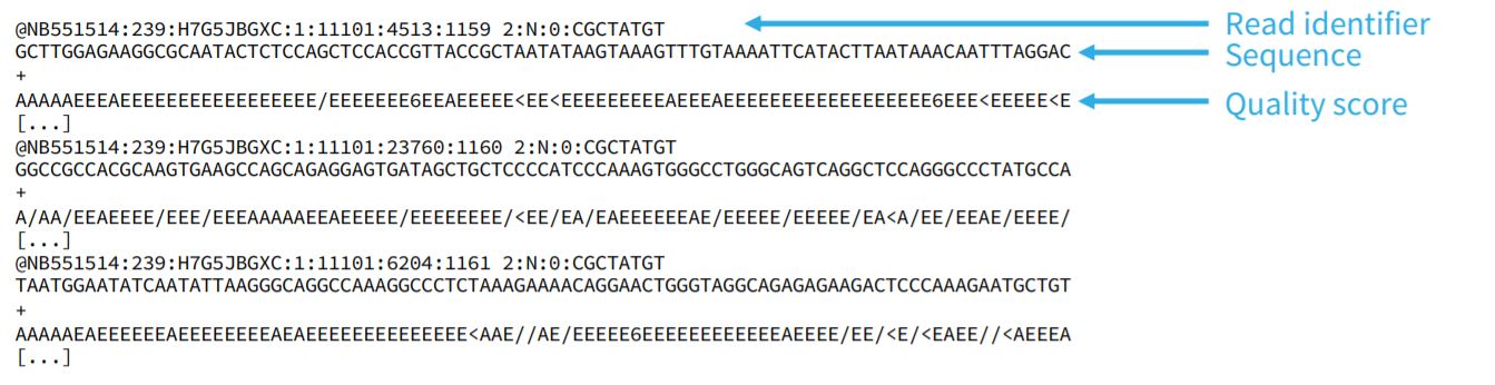
FIGURE 3.3: Structure of a FASTQ file

Each FASTQ file contains three parts. The first line of the FASTQ file that starts with @, contains the read identifier, which indicates the position on the flowcell. The DNA sequence starts from the second line. And the line comes before another read identifier contains the per-base sequencing quality score (also called PHRED score). The formula of the PHRED score is given below where P is the “Probability of base calling error”.

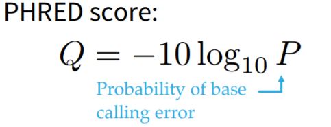
FIGURE 3.4: The formula of the PHRED score

3.1.2 Sequencing Quality : FASTQC tool

Sequence quality can be determined by FASTQC tool. FASTQC tool provides simple quality control check on raw sequence data that comes from high throughput sequencing pipelines. Anders (2010)

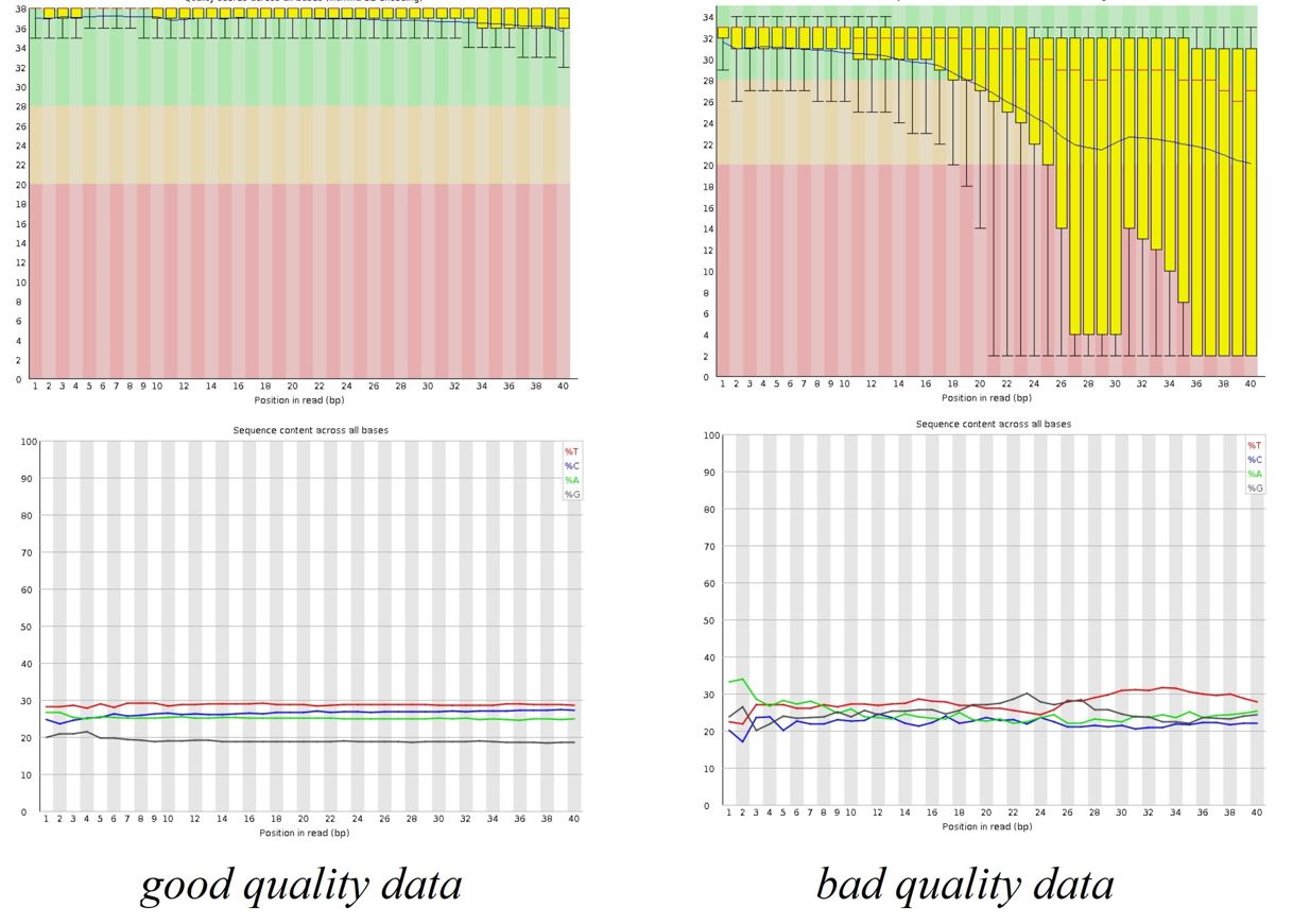
FIGURE 3.5: FASTQC Results

FASTQC tool provides:

• Summary statistics (number of reads, …)
• Sequencing quality summaries
• Sequence biases
• Duplicate reads
• Sequence contamination (adapters, etc.)

3.1.3 Read trimming

Sequencing data analysis pipelines modify the read sequences produced by a sequencer. There may be sequence biases due to structural oligonucleotides (adapters, etc.) and low-quality sequences. Trimming at reading ends is done as the first operation in a pipeline to avoid sequence biases.

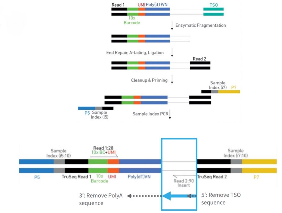
FIGURE 3.6: High-throughput sequencing pipeline scheme

There are several softwares present to apply trimming, frequently used ones are:

• CellRanger
• cutadapt
• Trim Galore!
• SeqPurge
• trimmomatic

3.2 Demultiplexing

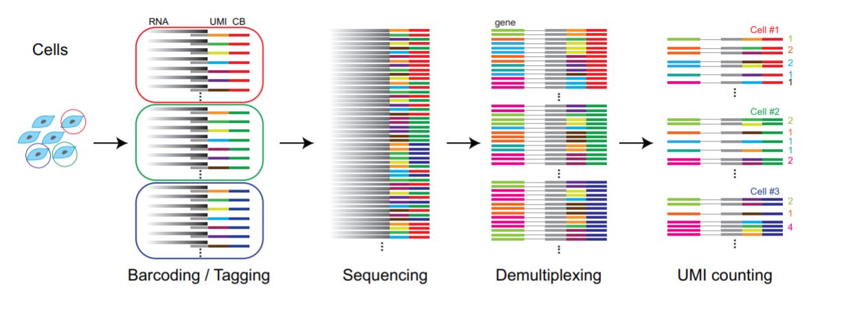
FIGURE 3.7: Data processing pipeline workflow.

Although the high-throughput sequencing methods provides data with good quality, errors via PCR can be introduced when preparing the library. When working with working with single-cell RNA sequencing data the initial cDNA libraries undergo PCR amplification multiple times. Thus, PCR errors are often introduced when preparing single-cell RNA sequencing library. Demultiplex is a simple sequencing error correction algorithm used to prevent this kind of errors. Zhang et al. (2018)

Demultiplexing indicates identification of cell barcodes, assigning cell-barcode to the associated reads and, filtration of cell-barcodes. If the data contains UMIs, UMI codes are mapped to the read name of the gene-body containing read. UMIs are counted for each cell and gene thus, duplicates are avoided. Genes are identified via sequence mapping. And, if the expected cell-barcodes are known, assigned barcodes are filtered accordingly.

Demultiplexing is done differently depending on the protocol and the pipeline of choice. In general, the data obtained from paired-end full transcript protocols and, Smart-seq2 are already be demultiplexed. If the data was not demultiplexed, you need to apply it yourself depending on the protocol used to produce raw data.

3.3 STAR: Ultrafast Universal RNA-seq Aligner

After trimming and, prof the data has good quality, the data needs to be mapped to the corresponding reference genome. This mapping process is called alignment and, it is necessary if we’re interested in gene expression analysis (eg. differential gene expression analysis, quantifying etc.) Kallisto and STAR are the most popular alignement tools. Dobin et al. (2013)

FIGURE 3.8: STAR workflow.(2017)

In summary, STAR searchs for the longest sequence in the data that is also present in the reference genome using an uncompressed suffix array (SA). This process is called seed searching. The longest matching sequences are called “the Maximal Mappable Prefixes (MMPs)”. The MMP side and the unread side are named as different seeds (eg seed1,seed2). After finding MMP, STAR searchs for the next the longest sequence. If an exact matching sequence for each part of the read is not found,the previous MMPs will be extended. And, if extending the previous MMPs oes not give a good alignment, then the poor quality or adapter sequence (or other contaminating sequence) will be soft clipped. These process is repeated for each for unmapped part of the read in forward and reverse directions. Dobin et al. (2013) STAR detects splicing events in this way, because of that,it also called splice aware aligner.

Then seeds are clustered by proximity to ‘anchor’ seeds (or uniquely mapping seeds) and, seeds are stitched together based on alignment score using dynamic programming. The scoring done based on matches, mismatches, insertions, deletions and splice junction gaps. Mistry, M. Freeman, B. Piper (2017)

3.4 Transcript Quantification: KALLISTO

FIGURE 3.9: Kallisto workflow.(2016)

While STAR is a read-alinger, Kallisto is a pseudo-aligner. That means, while STAR mapp reads to a reference genome, Kallisto mapps k-mers. Kallisto assign reads to transcripts without assigning specific positions for each base. Instead, it uses a Transcriptome de Bruijn Graph (T-DBG). A k-mer is a nucleotide sequence that length k derived from a read. Each transcript act as a path through the graph and, transcriptome reference represented as consecutive k-mers. Kallisto maps reads to splice isoforms rather than genes. Bray et al. (2016)

EM-algorithm is used to estimate transcript abundance and optimize compatibility (likelihood). Intersection of vertex compatibility classes indicates compatible transcripts.

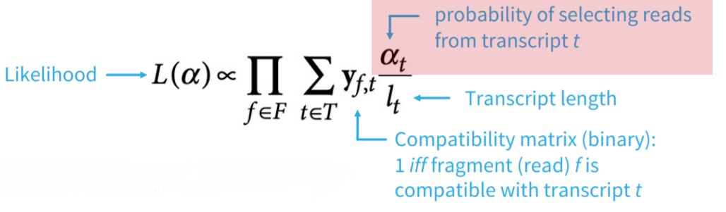
FIGURE 3.10: The EM algorithm formula.

K-mers of reads can be mapped to vertices using their exact matches (also called hashing). Read compatibility is found by matching the read mapping with transcript-induced paths (compatibility classes). It is much more faster than read-aligners. Pseudo-aligners can cope better with sequencing errors. For example, if k is sufficiently large, the error k-mers may not be part of the transcriptome and can be ignored.

3.5 The Single-Cell Data

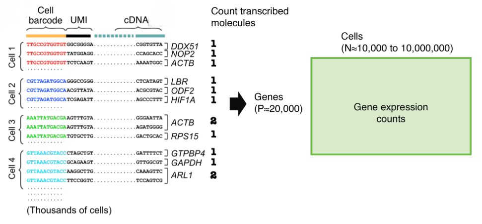
FIGURE 3.11: Representation of the single-cell count data

The raw counts of single-cell data are integers. The count matrices are sparse but, high dimensional. Therefore, feature selection and, dimensional reduction methods are necessary.

FIGURE 3.12: Representation of the sparse data (2009)

If the matrix has zero values for most elements, it can be considered as sparse data. The sparsity can be determined by the Number of Non-Zero (NNZ) ratio of elements. If the NNZ ratio is above 0.5 data can be considered as sparse data.

FIGURE 3.13: Representation of the Coordinate Matrix (COO) (2009)

To save memory, the sparse data can be stored in a coordinate matrix (COO). Only the non-zero elements stored as vectors and their respective indices in a COO. Thus, more efficient and less biased computation can be done on data.

FIGURE 3.14: Compressed Sparse Row (2009)

The Compressed Sparse Row (CSR) format is designed for more efficient indexing and computation and, it can be considered as “read-only”. The data (x) within the CSR consist of non-zero elements, index (i).

• Length = length of x
• Column indices of non-zero data

FIGURE 3.15: Compressed Sparse Column (2009)

Compressed Sparse Column (CSC) works exactly the same as CSR. But, instead of row based index,CSC has column based index pointers.

Pointers (p):

• Length = number of rows + 1
• Cumulative number of non-zero elements
• Differences indicate number of non-zero elements per row

3.6 Data normalization

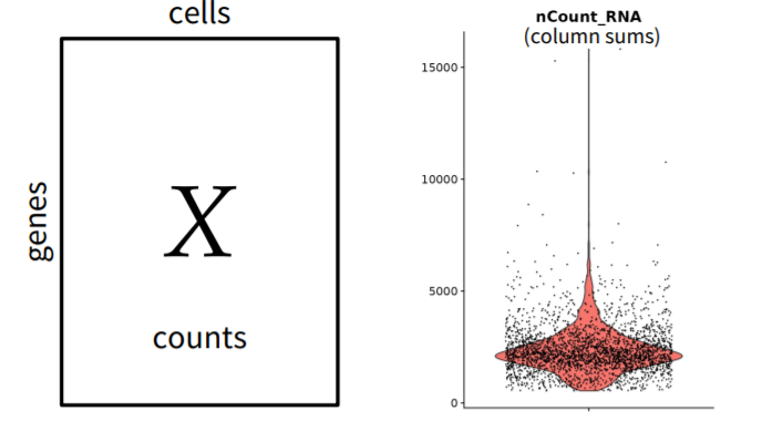
FIGURE 3.16: Single-cell sequencing counts

Single-cell sequencing data needs to be normalized to make quantifications comparable across cells and, mitigate cell-specific coverage biases. There are several methods present for normalizing the single-cell sequencing data. Hafemeister and Satija (2019)

1. Within-sample normalization.

FIGURE 3.17: Within-sample normalization formulas.

2. Non-linear normalization

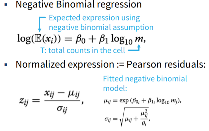
FIGURE 3.18: Non-linear normalization formulas.

3. Scaling: z-score

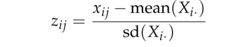
FIGURE 3.19: Scaling: z-score formula.

• Scale genes to mean 0 and variance 1
• Weight genes equally in downstream analysis
• Often used for visualization

4. Advanced methods for computing scaling factors

• DESeq, edgeR: pseudo-reference sample
• scran: robustness through pooling and deconvolution of cells
• sctransform:
  • Can incorporate other covariates besides total counts for batch correction
  • Avoid overfitting by regularization of fitted parameters over all genes

3.7 Dealing with Batch Effects

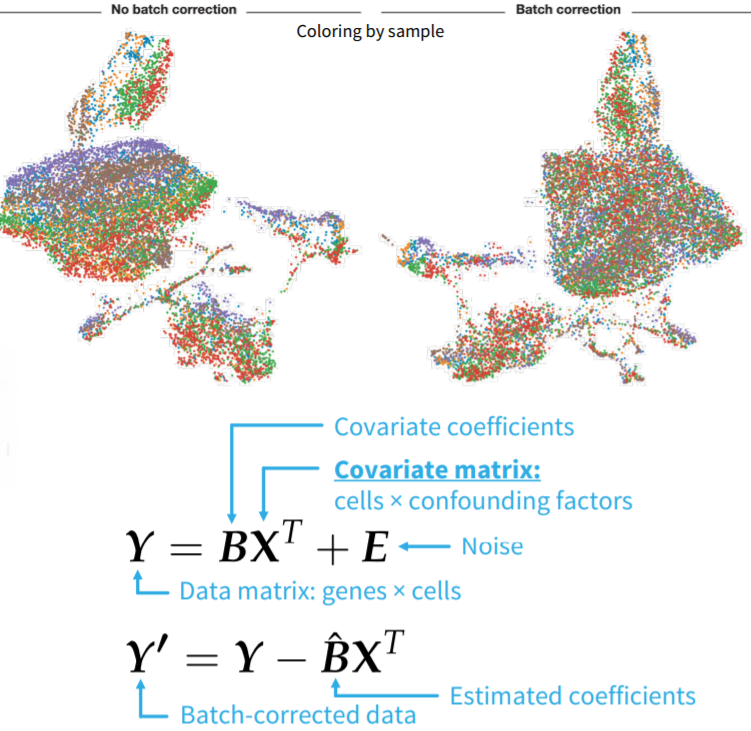
FIGURE 3.20: Representation of batch effect and, the ComBat formula.

There may be variations in the single-cell sequencing data due to confounding factors. These variations are called batch effects. Ideally, batch effects needs to be identified and corrected. Batch effects can be identified in exploratory analysis (dimensionality reduction, clustering, etc.) if adequate annotation is provided. Identified batch effects can be corrected by simple linear models (eg ComBat: empirical Bayes approach). The confounding factors that may cause batch effects are listed as below:

• Cell collection date

• Instruments and protocols used

• Cell environments

• Genetic population

• Factors that are not the focus of the analysis

• NOTE: Batch effects can only be corrected for if experiments are designed in a non-confounded way.

  • Sample groups need to be split across experimental batches

3.8 Data cleanup (filtering)

Along with the sparsity, single-cell sequencing data may contain uninformative data. This kind of uninformative data may be due to several reasons such as dying cells, cells with broken membranes and, doublets. These conditions are examples of outlier barcodes. We need to filter the data to remove the uninformative data. Filtration is done by removing the cells using metric thresholding ,removing genes and, removing droplets.

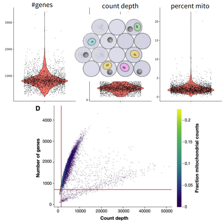
Remove cells using metric thresholding: * Number of reads per cell * Number of genes detected per cell * Mitochondrial read fraction (indicates the death and dying cells)

Remove genes * Genes expressed in only few cells * Not all genes might be relevant in all contexts (e.g.mitochondrial and ribosomal genes)

3.9 Empty Droplets

One barcode should correspond to one cell, but barcodes may not tag any cell (empty droplet) or, barcodes may correspond to multiple cells (multiplets, doublets). when removing droplets,the goal is to remove barcodes not corresponding to actual cells and, retain barcodes corresponding to actual cells with low RNA content. Lun et al. (2019)

The simplest way to remove droplets is setting a threshold on UMI counts.

• 99th percentile (minus 10%) of expected number of cells
• Filter based on elbow (knee) plot

EmptyDrops ambient testing is another option.

• Fit “ambient distribution” using barcodes below a threshold T
• Statistically test barcodes whether they significantly deviate from the ambient distribution
  • Good-Turing Smoothing algorithm to test deviation from multinomial (Dirichlet) distribution over all genes

Or, Combine ambient testing with thresholding: add high-UMI count barcodes as true cells.

3.10 Doublet detection and removal: demuxlet

FIGURE 3.21: Doublet detection with demuxlet (2018)

demuxlet is a method that leverages genotype information to detect doublets in genetically diverse cell populations. For each droplet, it uses the likelihood of genotyping calls to infer whether the droplet is a singlet or a doublet. The process involves:

• Maximum likelihood estimation of genotype matches
• Modeling doublets as a mixture of two genotype profiles
• Computing posterior probability for doublet classification

This approach is powerful when donor genotypes are known and enables reliable assignment of cells to individuals in multiplexed samples.

---

3.11 Doublet detection and removal: DoubletFinder

FIGURE 3.22: Doublet detection with DoubletFinder (2019)

DoubletFinder detects doublets by simulating artificial doublets and using a k-nearest-neighbor (KNN) classifier in PCA space. Steps include:

• Normalizing data and selecting variable genes
• Simulating doublets by merging transcriptomes
• Embedding into PCA space
• Computing proportion of artificial nearest neighbors (pANN)
• Classifying top cells with highest pANN as doublets

Parameter tuning (e.g. expected doublet rate) improves sensitivity.

---

3.12 Doublet detection and removal: Scrublet

FIGURE 3.23: Doublet detection with Scrublet (2019)

Scrublet is a Python-based tool that uses simulation and distance-based metrics:

• Simulates doublets by summing transcriptomes
• Embeds cells into PCA space
• Builds KNN graph and calculates doublet score
• Thresholds doublet score to identify doublets

Unlike demuxlet, Scrublet does not require genotype data and can be used with standard single-cell datasets.

---

3.13 Issues of the Single-Cell Data

FIGURE 3.24: Challenges in single-cell RNA-seq data (2014)

Single-cell data presents challenges:

• High sparsity due to dropouts
• Low coverage for some genes
• Technical noise and overdispersion
• Biological variability

Common strategies to address these issues:

• Normalization and scaling
• Filtering low-quality cells/genes
• Imputation or pseudobulk aggregation

These steps ensure more accurate downstream analysis like clustering or differential expression.

3.14 Data imputation / Data Smoothing

We already mentioned that single-cell data is noisy due to missing data and stochastic transcription. Missing values can be imputed via several methods, this process called data smoothing (eg data imputation).

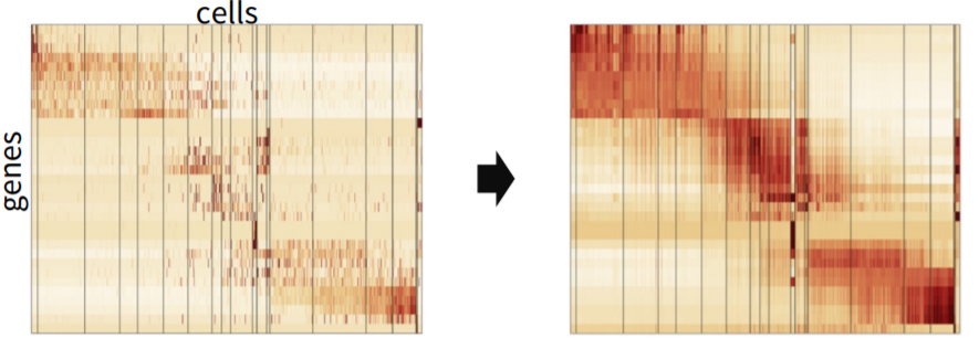
FIGURE 3.25: Representation of Data imputation / Data Smoothing in single-cell RNA-seq data

Imputation may be beneficial however, we must be careful with over smoothing. Over smoothing indicates false positives in differential analysis or artificial clusters. To detect over smoothing, downstream analysis on smoothed data needs to be carefully considered. Andrews and Hemberg (2018)

Here are the most popular imputation tools/softwares:

• scImpute: log-normal model detects dropout events and imputes using profiles from similar cells
• SAVER: negative binomial distribution modeling
• Knn-smooth: nearest neighbors
• dca: autoencoder
• MAGIC: diffusion
• netSmooth

3.15 MAGIC (Markov Affinity-based Graph Imputation of Cells)

FIGURE 3.26: Imputation with MAGIC (2018)

MAGIC is one of the sophisticated imputation/smoothing methods. MAGIC assumes that neighbors are informative. In summary, MAGIC algorithm calculates the gene scores signal across neighbors (nearby) cells and, impute gene scores based on this signal. The overall MAGIC workflow is given below.

FIGURE 3.27: The MAGIC workflow (2018)

MAGIC calculates the distance between neighbors and, the affinity of the neighbors. Then, learns from this manifold data with the implemented manifold learning algorithm. As a result, MAGIC construct a graph and, use it to impute the features. Dijk et al. (2018)

FIGURE 3.28: The formulas used in MAGIC imputation (2018)

References

10xGenomics. 2019. “Single-Cell RNA-Seq: An Introductory Overview and Tools for Getting Started. Retrieved 06-08-2019. https://community.10xgenomics.com/t5/10x-Blog/Single-Cell-RNA-Seq-An-Introductory-Overview-and-Tools-for/ba-p/547.” 10xGenomics, 5–9. https://www.10xgenomics.com/blog/single-cell-rna-seq-an-introductory-overview-and-tools-for-getting-started.

Anders, Simon. 2010. “Babraham Bioinformatics - FastQC A Quality Control tool for High Throughput Sequence Data.” https://www.bioinformatics.babraham.ac.uk/projects/fastqc/.

Andrews, Tallulah S., and Martin Hemberg. 2018. “False signals induced by single-cell imputation.” F1000Research 7: 1740. https://doi.org/10.12688/f1000research.16613.1.

Bray, Nicolas L., Harold Pimentel, Páll Melsted, and Lior Pachter. 2016. “Near-optimal probabilistic RNA-seq quantification.” Nature Biotechnology 34 (5): 525–27. https://doi.org/10.1038/nbt.3519.

Dijk, David van, Roshan Sharma, Juozas Nainys, Kristina Yim, Pooja Kathail, Ambrose J. Carr, Cassandra Burdziak, et al. 2018. “Recovering Gene Interactions from Single-Cell Data Using Data Diffusion.” Cell 174 (3): 716–729.e27. https://doi.org/10.1016/j.cell.2018.05.061.

Dobin, Alexander, Carrie A. Davis, Felix Schlesinger, Jorg Drenkow, Chris Zaleski, Sonali Jha, Philippe Batut, Mark Chaisson, and Thomas R. Gingeras. 2013. “STAR: Ultrafast universal RNA-seq aligner.” Bioinformatics 29 (1): 15–21. https://doi.org/10.1093/bioinformatics/bts635.

Eding, Matt. 2009. “Sparse Matrices.” In, 419–44. https://doi.org/10.1201/9781439811481.ch20.

Hafemeister, Christoph, and Rahul Satija. 2019. “Normalization and variance stabilization of single-cell RNA-seq data using regularized negative binomial regression.” Genome Biology 20 (1): 1–15. https://doi.org/10.1186/S13059-019-1874-1/FIGURES/6.

Kang, Hyun Min, Manasa Subramaniam, Sheila Targ, Mai Nguyen, Lenka Maliskova, Erin McCarthy, Emily Wan, et al. 2018. “Multiplexed Droplet Single-Cell RNA-Sequencing Using Natural Genetic Variation.” Nature Biotechnology 36 (1): 89–94. https://doi.org/10.1038/nbt.4042.

Kharchenko, Peter V, Lev Silberstein, and David T Scadden. 2014. “Bayesian Approach to Single-Cell Differential Expression Analysis.” Nature Methods 11: 740–42. https://doi.org/10.1038/nmeth.2967.

Lun, Aaron, Samantha Riesenfeld, Tallulah Andrews, The Dao, Tomas Gomes, and John Marioni. 2019. “EmptyDrops: Distinguishing Cells from Empty Droplets in Droplet-Based Single-Cell RNA Sequencing Data.” Genome Biology 20 (March): 63. https://doi.org/10.1186/s13059-019-1662-y.

McGinnis, Christopher S, Lauren M Murrow, and Zev J Gartner. 2019. “DoubletFinder: Doublet Detection in Single-Cell RNA Sequencing Data Using Artificial Nearest Neighbors.” Cell Systems 8 (4): 329–337.e4. https://doi.org/10.1016/j.cels.2019.03.003.

Mistry, M. Freeman, B. Piper, M. 2017. “Alignment with STAR | Introduction to RNA-Seq using high-performance computing.” https://hbctraining.github.io/Intro-to-rnaseq-hpc-O2/lessons/03_alignment.html.

Wolock, Samuel L, Ramon Lopez, and Allon M Klein. 2019. “Scrublet: Computational Identification of Cell Doublets in Single-Cell Transcriptomic Data.” Cell Systems 8 (4): 281–291.e9. https://doi.org/10.1016/j.cels.2018.11.005.

Zhang, Xiannian, Tianqi Li, Feng Liu, Yaqi Chen, Jiacheng Yao, Zeyao Li, Yanyi Huang, and Jianbin Wang. 2018. “Comparative Analysis of Droplet-Based Ultra-High-Throughput Single-Cell RNA-Seq Systems.” Molecular Cell 73 (November). https://doi.org/10.1016/j.molcel.2018.10.020.